Spiking Neural Networks on Neuromorphic Processors

For the first part of our exercise, we will dive into the remarkable world of biological neurons. Neurons are cells consisting of mostly water, ions, amino acids and proteins with unique electrochemical properties. They are the primary functional units of the brain. Our thoughts, perceptions and memories are the results of molecular movement across neural membrane and the synaptic transmissions between these neurons. Understanding neurons and neural computation can help illuminate how our rich mental experiences are constructed and represented, the underlying principles of our behavior and decision making, as well as provide biological inspiration for new ways to process information for artificial intelligence.

This page will be an interactive overview of biological neurons, by no means intended to be comprehensiveThere are several types of neurons in the brain e.g. pyramidal neurons, interneurons etc. and some rare types of neurons that do not spike e.g. non-spiking neurons in mammalian peripheral nervous system.. However, we hope it provides you with a smooth introduction about the basic working principles of biological neurons with an interactive model that lets you play with different model parameters.

Primer: Biology of the Neuron

Before we dive into mathematical model of an ideal spiking neuron, we should first take a brief tour of the biology of a neuron, it all its glory (you might be familiar with this part if you've taken other Neuroscience courses).

Anatomy of a Neuron

The first thing to appreciate about neurons is their specialized morphology, i.e. their form and structure. It allows them to receive information from more than $10^4$ mostly neighbouring cell bodies and communicate rapidly over long distances, sometimes from the spinal cord to the feet (up to a meter!). In the mammalian cortexThe cerebral cortex is the 2-3 mm thick outermost layer of the human brain., the connectivity of neurons are so dense that several kilometers of 'wiring' can be found in a cubic milimeter.

A typical spiking neuron can be divided into three different compartments: dendrite (input), soma (processing unit) and axons (output).

Drawing of a Purkinje cell from cat's cerebellar cortex, by Santiago Ramon y Cajal . Notice the complexity and number of dendrite branches.

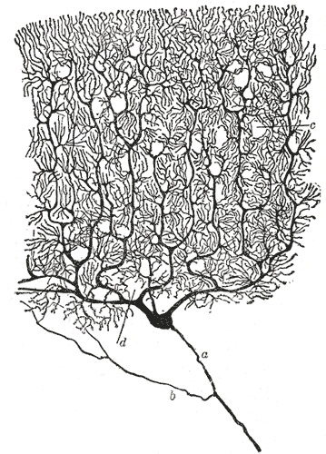
Neurons receive signals from other neurons through synapses located – not exclusively – on their dendritic tree, which is a complex, branching, sprawling structure. If you are wondering what the king of dendritic complexity is, that would be the Purkinje cell, which may receive up to $10^5$ other connections. Dendrites are studded with dendritic spines – little bumps where other neurons make contact with the dendrite. Signals from the dendrites propagate to and converge at the soma – the cell’s body where nucleus and other typical cell organells live.

Anatomy of a neuron.

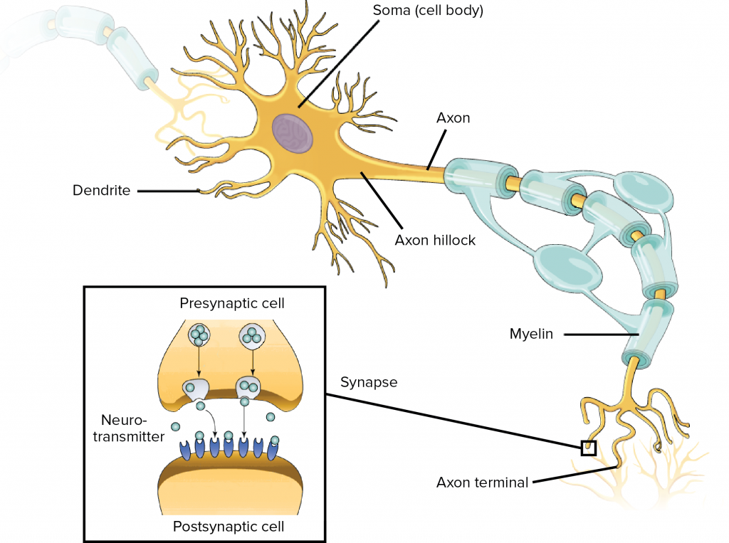
Coming off the soma is the axon hillock which turns into the axon. The axon meets other neurons at synapses. It allows a neuron to communicate rapidly over long distances without losing signal integrity. To allow signals to travel rapidly, the axon is myelinated – it is covered with interspersed insulators which allows the neuron’s signal to jump between insulated sections. To allow the signal to maintain integrity, the neuron signal in the axon is ‘all-or-nothing’ – it is a rather bit-like impulse, which we will discuss next.

Physiology of a Neuron

The second thing to appreciate about neurons is their specialized physiology — that is the cellular functions of neurons. The most striking feature of neural cellular function is the action potential, or "spikes". This is the mechanism which allows neurons to transmit information reliably over long distances without the transmission attenuating.

It is important to remember that neurons live in an extracellular solution of mostly water, salts and proteins. The forces caused by the movement of salts into and out of the cell and the different concentrations of these salts is the physical basis of the neuron’s remarkable behavior. There are sodium-potassium pumps which move sodium out of the cell and potassium in, so that the concentration of sodium outside the cell is higher than inside and the concentration of potassium outside the cell is lower then inside.

An action potential is a discrete event in which the membrane potential rapidly rises (depolarization) and then falls (polarization). This discrete event is all-or-nothing, meaning that if an action potential occurs at one part of the neurons membrane, it will also occur in the neighboring part, and so on until it reaches the axon terminal. Action potentials typically have an amplitude about 100 mV and duration of 1-2 ms. They do not tend to travel backwards, because, once a section of the membrane has fired an action potential, electrochemical-forces hyper-polarize the region of membrane while the channels which were previously open close and become inactive for some duration of time.

The action potential is the result of different types of ions traveling across the cell membrane through channels and the activation and inactivation of those channels on different time scales. A classic action potential occurs as follows:

1. Equilibrium. The neuron’s equilibrium membrane potential is near -70 mV — roughly the Nernst Equilibrium of $E_{K^{+}} \approx-75$ Nernst equation is a mathematical relationship that predicts the equilibrium potential across a membrane that is permeable to only one ion.. At equilibrium, inward and outward ionic flux are balanced. Net change is zero.
2. Depolarization. Incoming excitatory signals depolarize the membrane. Quick-to-respond voltage gated $Na^{+}$ channels are activated causing $Na^{+}$ to rush in and increase the membrane potential. Slower-to-respond $K^{+}$ channels open, and $K^{+}$ rushes out, pushing the membrane potential lower.
3. Amplification If the neuron becomes more stimulated or is stimulated rapidly, many more $Na^{+}$ channels are activated than $K^{+}$ channels. This causes a feedback loop where the influx of $Na^{+}$ causes more $Na^{+}$ channels to activate.
4. Repolarization. Eventually the membrane potential is near the Nernst Equilibrium of $Na+$ as the sodium channels are maximally open. The slower $K^{+}$ channels catch up to $Na^{+},$ which repolarizes the membrane potential. Meanwhile, the $Na+$ channels become inactive.
5. Hyperpolarization. $K^{+}$ channels are open while $Na^{+}$ channels are inactive, causing the membrane potential to dip below its typical equilibrium point, near the $K^{+}$ Nernst equilibrium.
6. Refractory Period. The $Na^{+}$ channels, take a while to being to become deinactivated, meaning after an action potential, they remain incapable of opening again for a period of time. The period in which most $Na^{+}$ channels is called the absolute refractory period (the neuron cannot spike no matter the strength of the stimulus) while the period in which many $Na^{+}$ channels are inactivated is called the relative refractory period (the neuron can spike given a sufficiently strong stimulus).

As we will see below, there exist different neuron models that capture the essence of an action potential mechanism with varying details. But, the general working principle still holds: neuron takes spike inputs from other neurons with its dendrites, performs a non-linear processing at soma - if the total arriving input is higher than a certain threshold it generates an action potential. The action potential is then transferred to other neurons using its axons.

Spike Trains

Spikes are the language of neurons and we usually deal with a series of spikes. We can formally define them with:

\[\rho(t)=\sum_{i=1}^{k} \delta\left(t-t_{i}\right)\]

where an impulse is described with a dirac delta function (which is convenient for representing discrete events):

\[\delta(t)=\left\{\begin{array}{ll}1 & \text { if } \mathrm{t}=0 \\ 0 & \text { otherwise }\end{array}\right.\]

Often, it is useful for analysis to assume spike trains are generated by a random processes due to existence of various noise factors. Assuming spikes are independent of each other, we can model the generation of the spikes as a Poisson process, in which we know the probability $n$ spikes occur in the interval $\Delta t$ :

\[P\{n \text{ spikes occur in } \Delta t\}=\frac{(r t)^{n}}{n !} \exp (-r t)\]

In practice, to generate spikes according to a Poisson point process, we generate a random number $r$ in a sufficiently small time interval e.g., 1 ms, such that only 1 spike should occur, and check whether $r$ is smaller than the firing rate $\Delta t$. However, we make sure that firing rate $\Delta t<1$. We are going to implement this process in the next exercise.

Simple Dynamical Models

If you weren’t constrained to thinking about ion channels — that is, if, for a moment, you could allow yourself to look past the wetware, the biological hardware — could you capture aspects of cell behavior relevant to neural computation while maintaining the simplicity needed for tractable analysis and simulation. The intuition behind Eugene Izhikevich’s simple model is that a good model needs first, a fast variable describing the membrane potential and second, a slow variable describing the recovery dynamics. The recovery variable does not need to explicitly represent a particular ionic current, rather it can describe the sum of all recovery currents. This has great benefits when simulating networks of neurons. Not only is the computational cost reduced by simplifying the dynamics to 2 variables described by relatively simple ordinary differential equations, one model can be used to represent a multitude of neural properties.

\[ \frac{d v}{d t}=0.04 v^{2}+5 v+140-u+I \] \[ \frac{d u}{d t}=a(b v-u) \] \[ \text { if } v \geq v_{\text {peak}}, \text {then }\left\{\begin{array}{ll} v & \leftarrow c, \\ u & \leftarrow u+d \end{array}\right. \]

Here, $u$ and $v$ are dimensionless variables, $a,b,c,d$ are dimensionless parameters, $t$ is time. The variable $v$ represents the membrane potential of the neuron and $u$ represents the membrane recovery variable which accounts for the activation of $K^{+}$ ionic currents and inactivate $Na^+$, basically provides the leaking effect. $I$ is the synaptic currents injected to soma.

Now it's time to play! You can adjust the model parameters below to simulate some known neuronal dynamics. We suggest you to check Izhikevich's Simple Model of Spiking Neurons paper to find proper model parameters for achieving regular spiking, intrinsically bursting, chattering, fast spiking etc.

Computational Properties of Neurons

Neurons decode information from other neurons, transform this information, and then encode information to other neurons in the form of spikes. The computational properties of neurons enable them to perform this operation. Below are some examples of computational properties (the list is by no means comprehensive).

Class 1, 2, and 3 Neurons

One way to look at the computational powers of neurons is to look at their F-I functions — that is, their gain functions. Hodgkin proposed 3 classes of neurons based on this metric, which are represented in the below figures:

This is an example of a class 1 neuron’s F-I curve. Notice the curve is smooth. These neurons are able to generate arbitrarily low frequency spike trains.

This is an example of a class 2 neuron. There is a discontinuous jump in firing rate. Type II neurons are not able to generate arbitrarily low frequency spike trains.

Class 3 neurons don’t have interesting F-I curves, since they fire only at the onset of an input. That is, they generate a single spike when given a constant input.

It should be said that there are many other ‘types’ of neurons. That is, there is more to neurons than their gain functions. In fact there is a project at the Allen Institute working on the lumping of neurons into types. They have an amazing open source brain cell database.

Integrators and Resonators

We can also consider whether neurons are either integrators or resonators. Integrators accumulate signals until their membrane potential reaches a well defined threshold. Closely timed signals are added together and have greater affect than when far apart. Integrators are coincidence detectors. Some integrators are Type 1 neurons.

This is an example of an integrator. The neuron integrates the constant input overtime.

Above is the phase portrait of a Simple Model. The vector field (black arrows) depict the trajectories throughout the state space, (2) the null clines (solid black lines) depict the points where a partial derivative is $0$, (3) the fixed point (black dot) where in this case all points evolve toward, and (4) the trajectory (red) showing a trajectory through the state space. Shown here is also a basin of attractionThe set of points in the space of system variables such that initial conditions chosen in this set dynamically evolve to a particular attractor. (blue area) in which all points tend toward a stable node (black point). The separatrixA separatrix marks a boundary between phase curves with different properties. (solid blue line) leads directly into the saddle pointA point of a function or surface which is a stationary point but not an extremum. (white point) and also defines the boundary of the basin of attraction.

Resonators resonate (oscillate) in response to incoming signals. Resonators do not necessarily have clearly defined thresholds. The threshold is fuzzy. Unlike integrators, resonators are most sensitive to a narrow band of frequencies. Resonators are coincidence detectors as well, but they are also frequency detectors. All resonators are type 2 neurons.

Above, is an example of an integrator. We are able to make a resonator neuron spike with three very small amplitude pulses. Since these pulses are at the right resonant frequency and push the membrane potential higher and higher. This is similar to swinging your legs in the right rhythm on a swing.

Above figure shows another example of resonator model dynamics.